Hello Haasoscope Pro backers and enthusiasts!
Thanks to you, we are more than halfway to our funding goal, with still a few weeks to go. If the project seems interesting to you, please consider backing it and you’ll soon have your very own GHz+ scope at the introductory campaign price! Also, please help spread the word to others who might be interested — social media, email, or just good old word of mouth.

For this week’s update, let’s take a look at the Haasoscope Pro "front-end:" all the analog magic between the BNC input and the ADC that digitizes the signal. When you hear "2 GHz oscilloscope", you might rightly wonder what kind of analog wizardry can possibly achieve such crazy bandwidth. As you’ll see, the real key was just to use some incredible components. Here’s the key part of the Haasoscope Pro schematics:

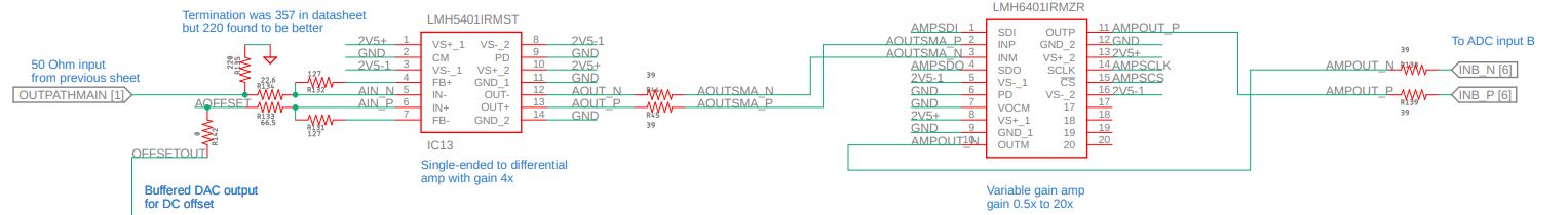
On the left, a 50 Ohm impedance signal is input. (This could be direct from a BNC input connector, but as we’ll see below the Haasoscope Pro does a few extra things between the BNC input and this 50 Ohm input.) After just a few resistors for impedance matching, this signal is fed into one input of the LMH5401 preamplifier. This incredible chip has 8 GHz of gain bandwidth product. We use it as a 4x gain, single-ended to differential amplifier. The other input to the chip is a (high bandwidth, low impedance, buffered) DC voltage from a DAC, so we can control the signal’s DC offset.

The differential output is then passed to the LMH6401, a 4 GHz bandwidth, variable gain amplifier. We use it to vary the signal gain by an extra factor of between -6 to 26 dB (~0.5x to ~20x), in 32 steps. The output of that amplifier is then fed directly into the ADC. With just those two components, we basically have a 2 GHz front-end!

To really have a fully functional oscilloscope front-end though, we need to be able to process the input signal in a few more ways. Here’s the schematics for one of the two channels, from the BNC input to the preamplifier input:

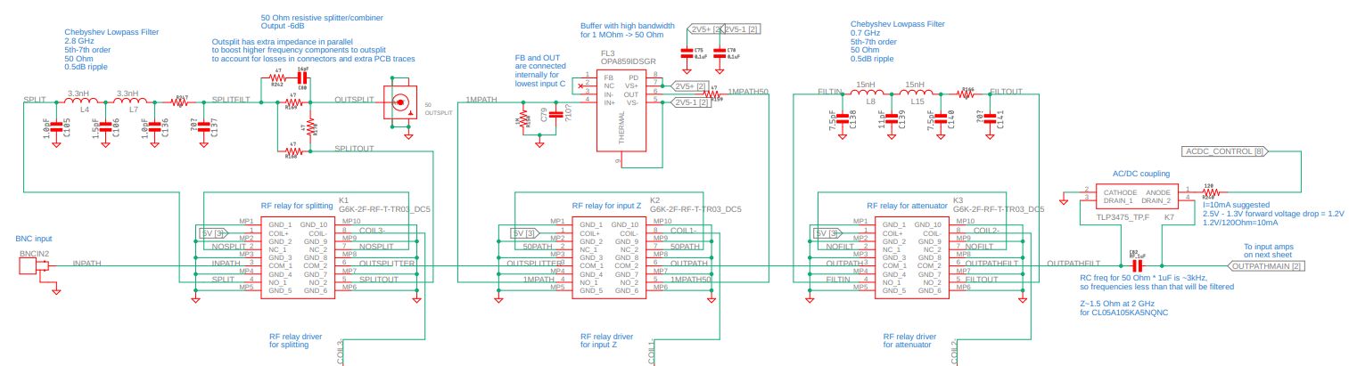
Right after the BNC input is a stage which can optionally split out half the signal power to an SMA output on the front, so you can send it to a second Haasoscope Pro for oversampling. This is only on channel One, since if you’re bothering to oversample the signal, you’re first going to be using the ADC in single channel mode to get the full 3.2 GS/s for the channel. The splitting is done by a simple resistive divider in the Delta configuration, with a bit of frequency compensation to make up for signal losses on the way to the second scope. Half of the signal is lost to heat, but that’s OK, we have amplifiers afterwards. (We’ll have more on oversampling using two Haasoscope Pro’s in a future update.)

This, and other options, are switched on or off by a relay. But not just any relay will do, as most will only have a few hundred MHz of bandwidth at best. We need special "RF relays". Here I settled on the Omron G6K-2F-RF-T, which is rated to 3 GHz, but really starts to degrade significantly after 2 GHz. But that’s good enough for us here, and already it’s ~$10 each. Better relays are available, but can easily be ~$100 each!

The next stage allows for switching to 1 MOhm input impedance, for using standard 10x passive probes. These probes inherently don’t have large bandwidth — the excellent ones recommended from the Haasoscope Pro product page are "just" 500 MHz probes. This is far from 2 GHz, so why bother with 1 MOhm impedance at all? Well, sometimes you just want to use 10x passive probes and don’t care about the bandwidth. But also, if we’re in two channel mode, we have "only" 1.6 GS/s per channel, and that’s not such overkill for 500 MHz of bandwidth.

I really like the way the Haasoscope Pro handles 1 MOhm impedance. The trick is to take in 1 MOhm input impedance, but then immediately turn it into a 50 Ohm signal, for processing just like a 50 Ohm input. This lets us reuse the same magical high bandwidth 50 Ohm amplifiers we use for a 50 Ohm input. We make use of another fantastic chip, the OPA859 op-amp, with up to 1.8 GHz of bandwidth. And importantly, the inputs are CMOS MOSFET inputs, meaning they are crazy high impedance, like 1 GOhm, with just 10 pA of input bias current. That means we can put a 1 MOhm input into it and not have the amplifier itself affect the input signal.

The following stage is a switchable anti-alias filter. This attenuates all frequencies above the Nyquist frequency (half the sampling frequency). Otherwise those higher frequencies will appear as lower frequency distortions in the signal after sampling. We use a 5th order LC Chebyshev filter to do the job. There’re three different anti-alias filters for three different cutoff frequencies, depending on the sampling rate being used, for two channels (1.6 GS/s), one channel (3.2 GS/s), or oversampling (6.4 GS/s).

The final stage is AC/DC switching. A capacitor does the DC blocking, letting through only signals with frequencies above 1/(2 $\pi$ RC). For us, R is 50 Ohm, so C needs to be as big as possible - we use 1 uF, giving a ~3 kHz cutoff. DC signals are let through by a photo-MOSFET when it is on. We need to make sure it doesn’t add capacitance and ruin bandwidth though, so the TLP3475 is used. We also need to make sure the capacitor doesn’t add significant impedance, something we don’t usually worry about - but at some large frequency every capacitor becomes an inductor, past its self-resonant frequency. Fortunately, Samsung provides data on their capacitors and, for the one we use, it is indeed an inductor at 2 GHz (with a self-resonant frequency around 10 MHz!), but its impedance is only ~1.5 Ohm at 2 GHz, so not significant compared to 50 Ohm.

That’s it! Thanks for reading this far, and thanks for your interest in and support of the Haasoscope Pro!