Project update 8 of 8
Production Status & Corner Blending Improvements
by Liam PowellProduction update
Many of the people reading this are probably most interested in production updates, so that’s where we’ll begin. Shipping of our samples to the EMC test lab is taking a while. Currently, the boards are stuck in customs. We cannot begin production until we know that the boards will meet all relevant standards. However, once testing is complete, we will be ready to begin production as soon as possible.
We have also updated our documentation for the final board that will be shipping: https://prunt3d.com/docs/hardware/prunt_board_3/
Corner blending update
We’ve also been working more on our improved corner blending system, so we’ll share more details on that in this update. This write-up is aimed at readers who remember high-school mathematics so if you have more in-depth knowledge you may want to skip over some of the background information below. We’ve attempted to include as much detail as possible while still making this accessible to all readers, feel free to contact us if you have any questions on details not included here.
Mathematical background
Vectors, length, and the dot product
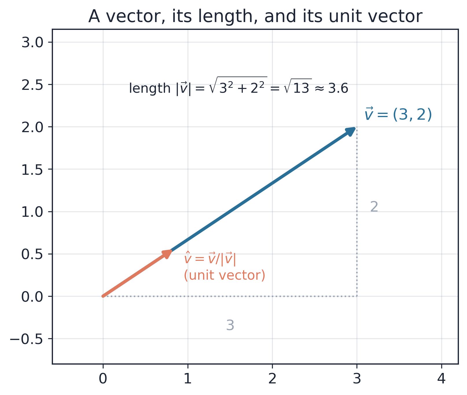
A vector can be thought of as an arrow, they are often represented as a list of coordinates. In 2D, (3, 2) means "3 across, 2 up". The length of this vector can be determined using the Pythagorean Theorem.
A unit vector is a vector of length 1, we use them when we just want a direction and not a length. You get one by dividing a vector by its own length.
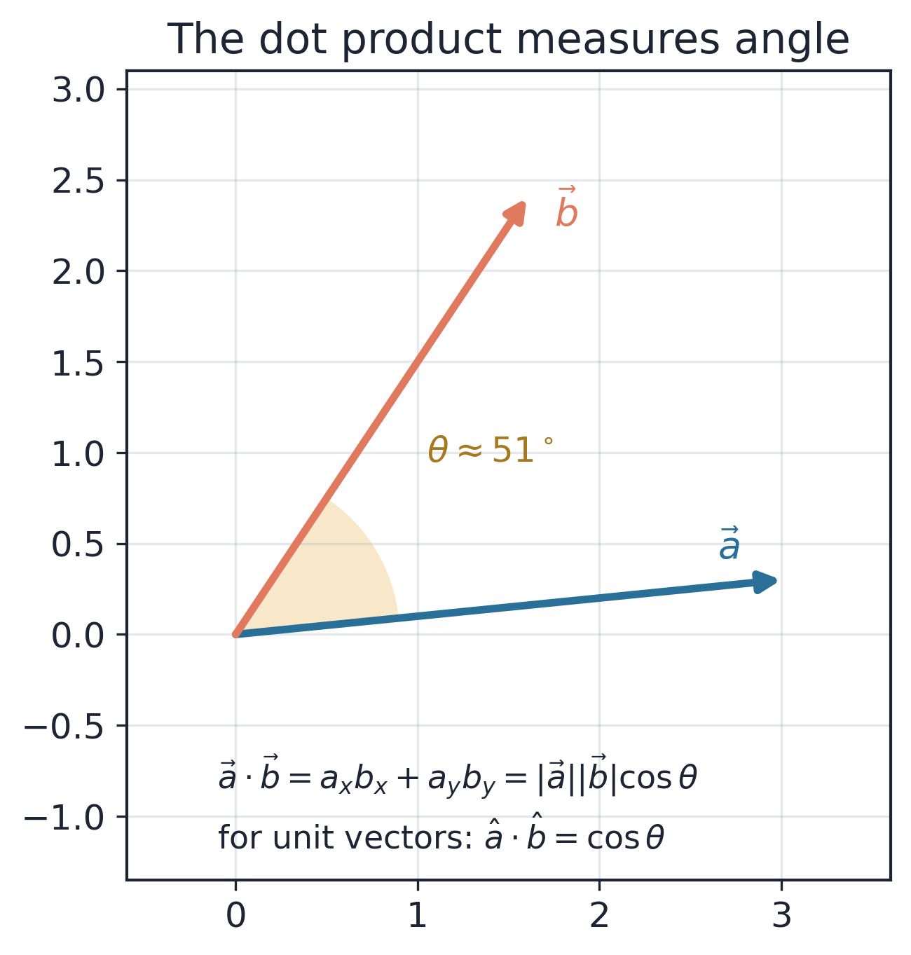
The dot product of two vectors multiplies matching components and adds them up. For example, for the vectors (a, b, c) and (x, y, z), the dot product is ax + by + cz.
An important property of the dot product is that it is equal to the product of the two vector lengths and the cosine of the angle between them. So for two unit vectors, the dot product is just the cosine of the angle between them.
Curves, tangents, and arc length
A parametric curve describes motion by giving position as a function of a single number. We use X(U), where the parameter U runs from 0 to 1. As U increases, X(U) traces out the path.
The derivative dX/dU is tangent to the curve. If you think of U as time, this is the velocity vector: its direction is the direction of travel and its length is the speed with respect to U.
The arc length, usually written as s, is the distance travelled along the curve. A curve is called unit speed, or arc-length parameterized, if it moves exactly one unit of distance per unit of parameter, i.e. |dX/ds| = 1 at every point on the curve.
Prunt stores blend curves using normalized arc length. If the full curve length is L, then s = LU and the unit tangent is T(U) = dX/ds = (1/L)dX/dU.
Most motion control systems, including Prunt, use a trajectory plan at their core, which tells us what distance we should be along a path at a given time. Once we have the distance that we need to be along the path, we need to take that number and convert it into our position on the path. A normalized unit-speed curve is well suited to this because finding a point at a given distance is as simple as X(D/L) where D is the distance and L is the arc length.
Derivatives and smoothness
A derivative measures a rate of change. The derivative of position is velocity, the derivative of velocity is acceleration, etc. for jerk, snap, and crackle. A motor can only push so hard, its force can only change so fast, and so on. If any derivative suddenly jumps, the machine gets a mechanical shock that shows up as a ringing artifact on the print surface. This lessens as the derivatives get higher. Prunt goes up to crackle, which is far enough for ringing to no longer be measurable.
Integration is the reverse of differentiation. If you know the velocity at every instant, integrating gives you the displacement. This is worth remembering as we will use this fact to turn a chosen set of tangents (directions) into a path that the printer can move along.
Polynomials
A polynomial is a sum of powers of a variable with fixed coefficients. For example, 12 + 34x + 56x² + …. Polynomials are easy to evaluate, easy to differentiate and flexible enough to take almost any smooth shape if you allow enough terms.
Building a curve from its tangents
Most curve drawing schemes, which rely on Bézier curves, choose the positions directly and find the tangents from that. Prunt instead does the opposite. Prunt starts with the tangent field (the direction of travel at each point) and then integrates that to get the position.
Why does it work this way? Because the constraints we care about the most are about directions. We want to leave in one direction, arrive in another direction, and keep the turning gentle. Controlling the tangent directly makes those constraints easy. It is more difficult to make the curve arrive at the exact point where the next segment starts, however the trade-off turns out to be worth it.
Unit vector tangents live on a sphere
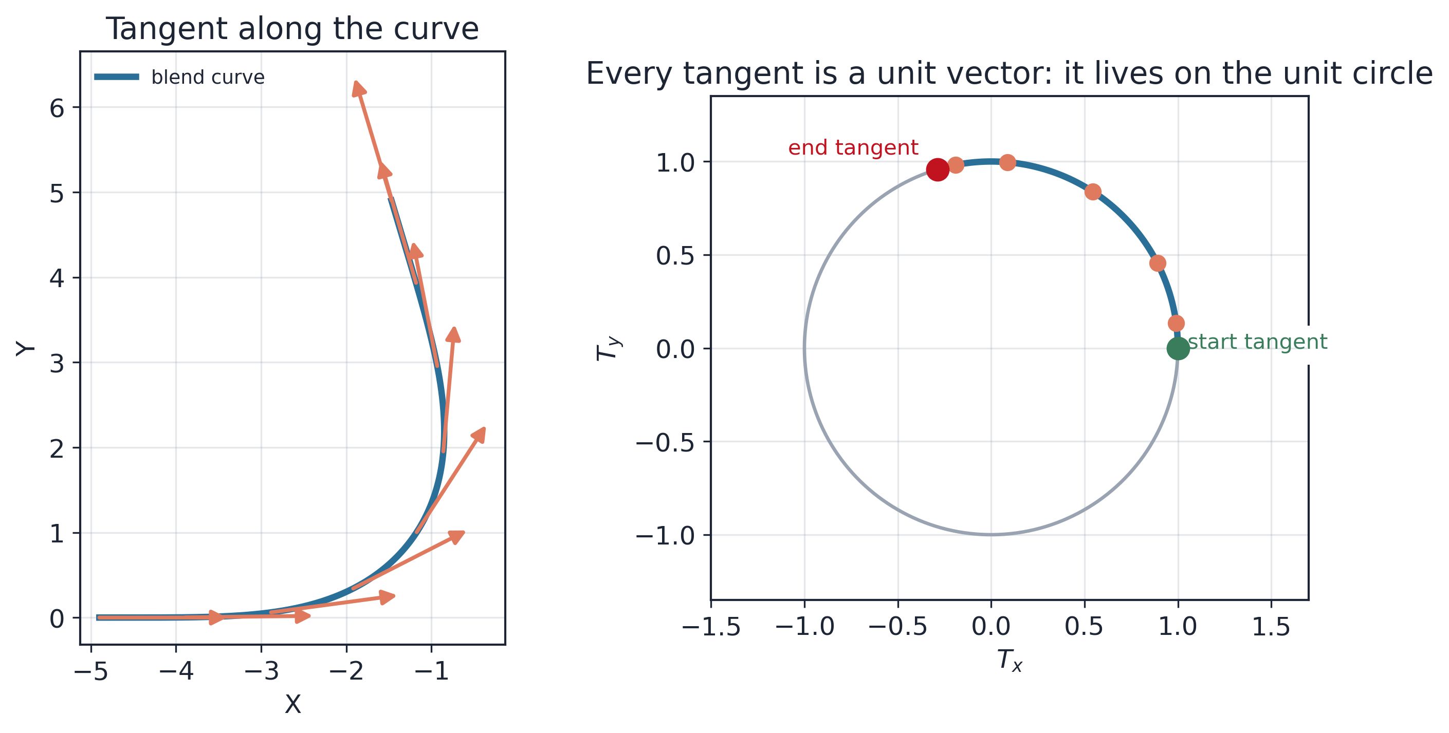
Unit speed curves have another interesting property which has not yet been covered. The tangent of a unit speed curve is a unit vector. The set of all unit vectors in the plane is exactly a unit circle. In ℝ⁴, which is the natural coordinate space of a printer with the XYZ axes plus the extruder axis, the unit vectors lie on a unit hypersphere (the 4-dimensional version of a sphere). Therefore, as we travel along a unit speed curve in ℝ⁴, the tangent traces a path on the surface of that hypersphere. Don’t worry about the fact that our curve uses a hypersphere, you only need to consider a curve on a 2D plane to gain an understanding of how our corner blender works.
The diagram below shows a curve on the left with its tangents drawn as arrows, on the right each of the same tangents is plotted as a point on the unit circle. Travelling along the curve corresponds to the tangent point sliding along the circle from the start direction to the end direction. Therefore designing the ℝ⁴ corner blend is the same task as designing a path along the surface of a hypersphere.
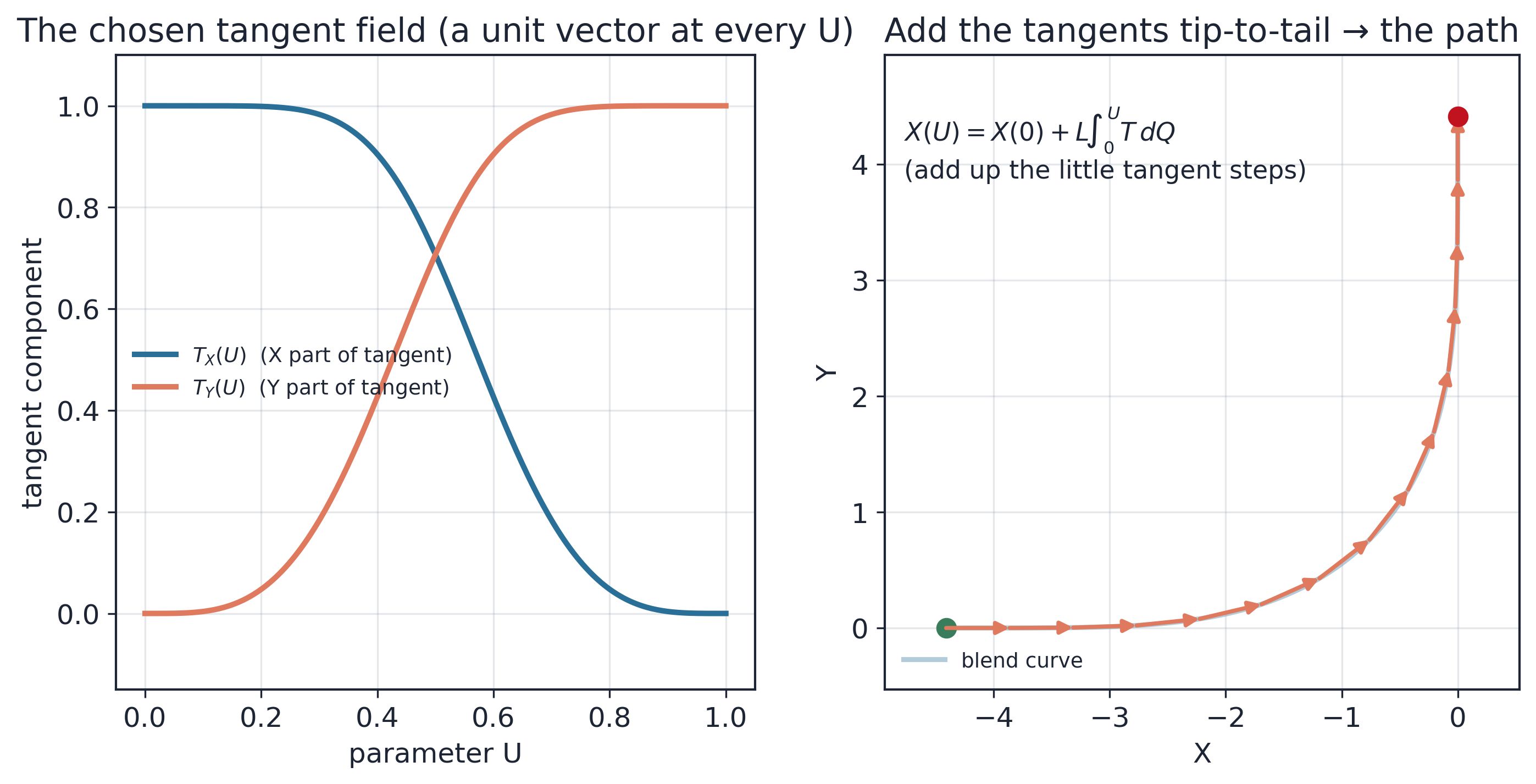
Once we have a tangent T(U) at every parameter value, we recover position by integrating, literally adding all the tangents: X(U) = X(0) + L ∫₀ᵁ T(Q)dQ where L is the total length of the curve.
In the below diagram the left panel shows a tangent field, the X part of the tangent starts at 1 (headed along +X) and goes to 0, while the Y part goes from 0 to 1 (heading along +Y). This gives us a quarter turn from +X to +Y. The right panel shows all the tangents as we increase U lined up from tip to tail, as they are when we add them all together. Of course in the actual implementation we do not add up tiny tangents, we instead have an equation which adds an infinite number of infinitely small tangents.
This reframing leaves one question: How do we choose a smoothly varying direction in ℝ⁴? Generally, a direction in ℝ⁴ can not just be represented as a single number as it can in 2D. When we use a unit vector to represent a direction, we have 4 numbers where the squares of those 4 numbers must sum to 1. This constraint is awkward to work with when trying to apply other constraints to get a smooth curve. The next section completely eliminates this issue.
Stereographic projection
We want to build the tangent field out of polynomials, however a tangent must be a unit vector, and polynomials do not naturally keep the length of unit vectors equal to 1. The way we avoid this issue is stereographic projection.
Stereographic projection is a way to flatten a sphere onto a plane. Stand at the north pole of a sphere and for any point draw a straight line from the north pole through to that point. Wherever the line crosses a flat chart placed somewhere below you, that is the point’s chart coordinate. Below is the 2D version, which shows a circle being projected onto a line. Note that it is impossible to draw a line from the north pole to itself, meaning that the north pole can not be represented on the chart.
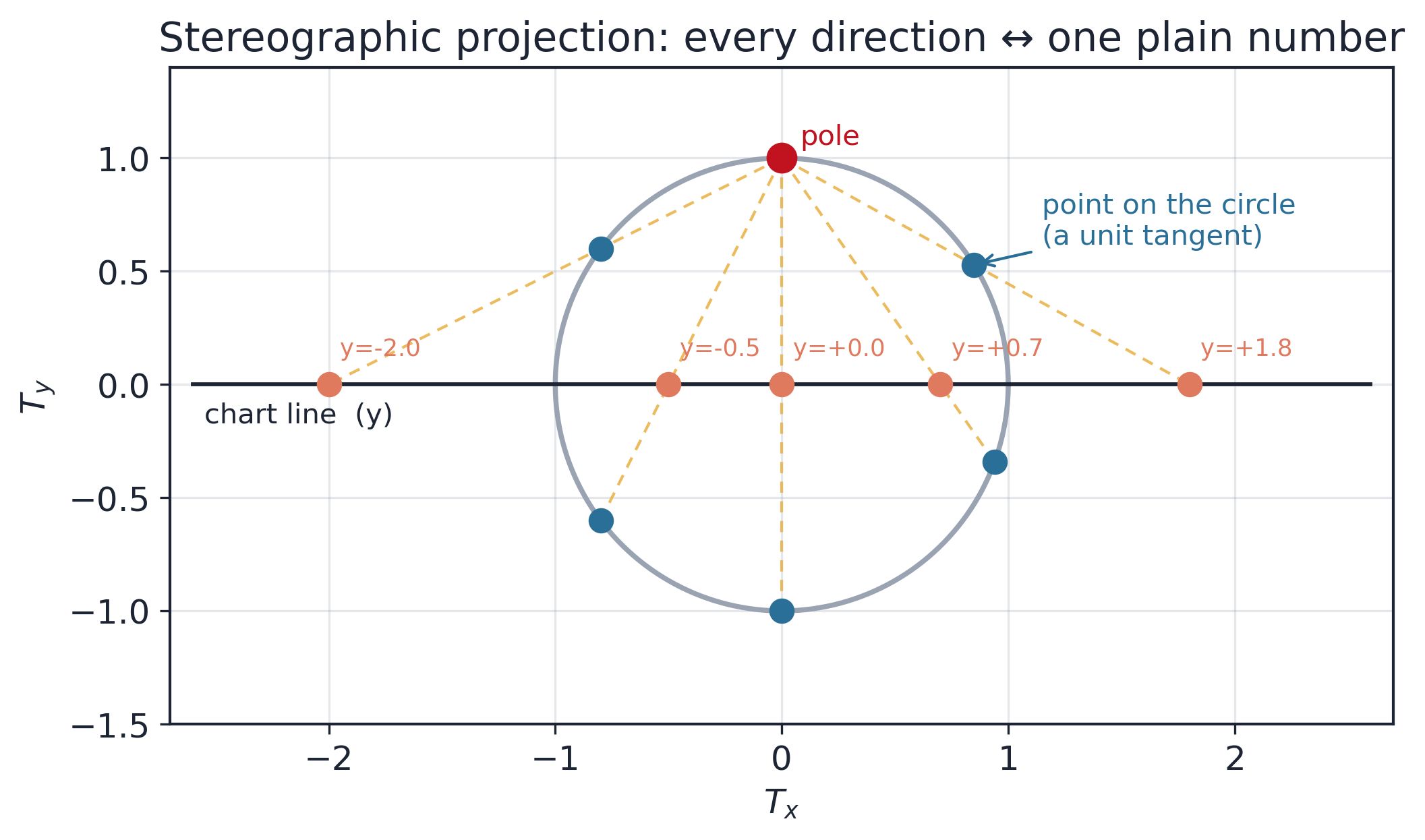
Every point on the circle maps to a plain number on the chart line. The reverse of this is also true, every number on the chart line maps back to a point on the circle.
The reverse direction is the one that we are most interested in: It means that we can take a polynomial which generates a point on the chart line and map that back to a point on the circle without the messy constraint that we need to keep the length equal to 1.
This same trick works in every dimension. The diagram above shows a circle projected onto a line, but we can also project a sphere onto a plane or a hypersphere onto a volume. Any point on the plane naturally becomes a point on the sphere, which is of course a unit vector. Similarly, any point in the volume naturally becomes a point on the hypersphere, which is also a unit vector. Essentially, describing a direction always costs one fewer number than the space that direction lives in, because its length is fixed at 1 and carries no information.
It is worth mentioning again that we cannot draw a line from the pole to itself. For the circle case, this would result in a point on the line at either infinity or negative infinity. We deal with this later on by setting up the coordinate system such that all tangents will sit far away from the pole, where the chart numbers stay small and well behaved.
To summarize the representation so far, our planned curve is stored as a polynomial Y(U). To find the tangent at parameter U, evaluate the polynomial and put the result through the stereographic representation formula. To find the position, integrate the tangent. So now the problem is the selection of a polynomial.
Selecting the tangent field
We now need to design the polynomial chart Y(U). There are three main areas to focus on:
- Select a sensible coordinate system.
- Make the ends match their neighbouring segments.
- Shaping the area between the two ends.
The local frame
Before we even start designing a polynomial, we first select an orthonormal frame. This consists of four mutually perpendicular unit vectors that act as a private set of axes for this one blend. The key constraint here is that one of the axes, which we will label as f₀, is aimed at the average of the incoming and outgoing tangents, as shown in the below diagram.
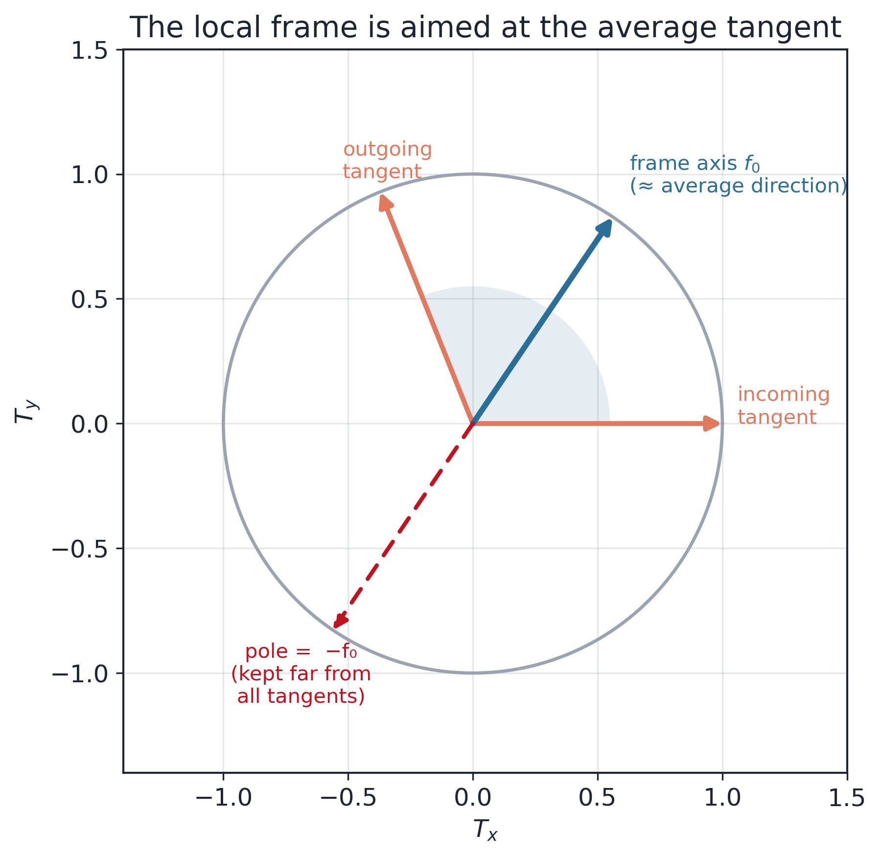
Because the pole of the stereographic chart sits at -f₀ and the blend is designed to keep its tangents in the area between the incoming and outgoing directions, every tangent we will need is far from the pole. This keeps the chart coordinates small and keeps arithmetic on them stable.
Matching the endpoints
At U = 0, the chart must have a value that corresponds to the incoming direction. At U = 1, the same applies for the outgoing direction. It is of course trivial to match just these points using lines. This however leaves a jump in the middle of the curve. Therefore, we need a way to blend between these two lines smoothly. Specifically, we need a continuous curve for derivatives all the way from velocity through to snap, leaving us with bounded crackle.
We also need to match the velocity, acceleration, jerk, and snap of the segments at both ends. This is trivial for lines, however things get more difficult for arcs. We won’t go into what the derivatives for different shapes are here as that is not important. What is important is that we need a way to match derivatives.
Hermite interpolation is the tool that we use to achieve this. It matches not only the values at both ends of the polynomial, but also a chosen number of derivatives at both ends. We will not go into much detail here, as we do not do anything special in regards to Hermite interpolation. In short, because the polynomial describes the tangent chart rather than position directly, we put values and their first 3 derivatives in for both ends. What we get out is a polynomial that matches the unit tangent and its first 3 derivatives at both ends. After integration, the path matches through snap. The below diagram shows the simple case where all endpoint derivatives are zero.
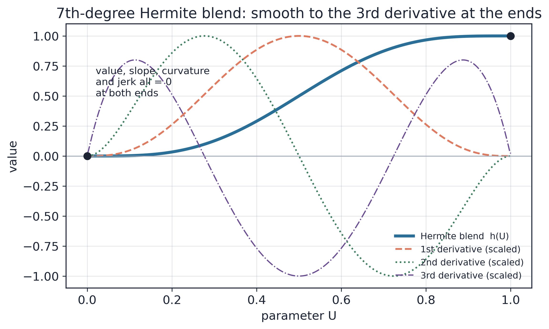
There is also some complexity around converting derivatives into the local frame, especially with derivatives that change depending on where on the incoming segment they sit. This is however a bit outside the focus of this update.
Interior shape
A Hermite blend, which only matches at the endpoints, is not particularly useful on its own. We also need a way to adjust the middle of the blend to get the shape that we want. To achieve this, we add extra polynomial terms, which are chosen so that they and their first three derivatives are zero at both ends. We call these interior shape modes.
Because each mode and its derivatives are zero at both ends, adding any amount of any mode change only changes the middle of the curve without disturbing the carefully matched endpoints. We won’t go into detail of how we use these modes here, as that may change over time and is very math-heavy.
Making the ends meet
There is one downside to our method as presented so far. We have chosen the tangent field so that the directions of the ends are perfect. However, the endpoint position is just whatever the integral happens to produce. In general, this is not the point that we need to reach. We must adjust the curve such that the integral lands exactly on the required endpoint. The diagram below shows the issue. Note that we cannot just scale the curve, as this would throw off all our carefully matched derivatives. Scaling the derivatives and then recomputing the curve would give us a completely different curve.
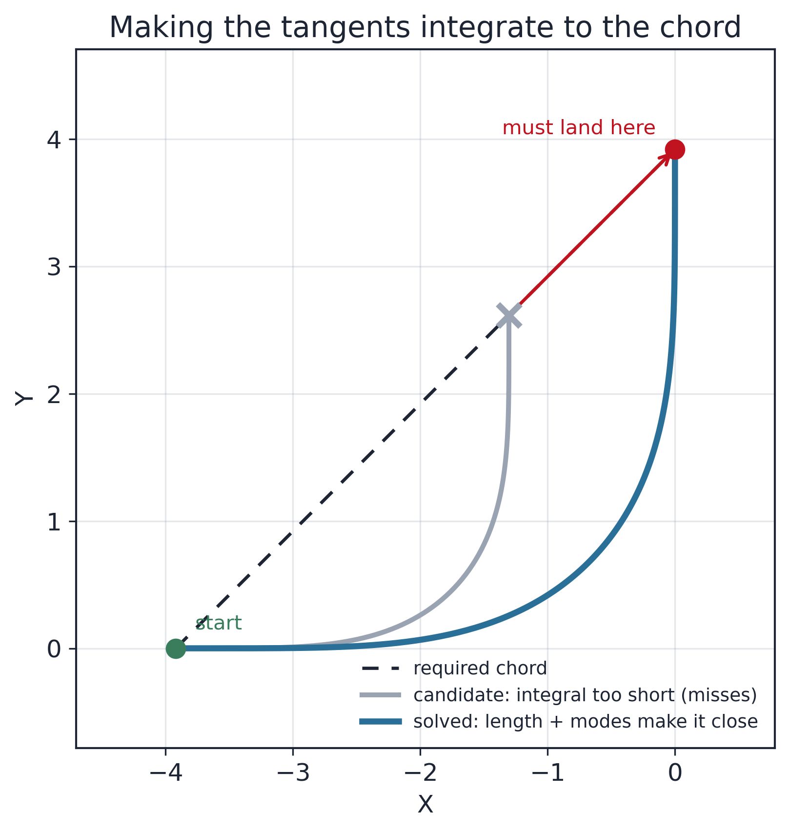
The way to solve this is to adjust some of the variables of our interior modes that were mentioned above. We, again, won’t go into too much detail here. In short, we choose four independent unknowns, which gives us one degree of control for each coordinate of the target point in the local frame.
Evaluating the curve
Now that we finally have our curve, we get back to the original problem. How do we take a tangential trajectory plan and convert it into positions on the curve both quickly and accurately? Because of the choices that we have made so far, we can now find our closed-form integral of the tangent.
Without going into too much detail, each tangent component is one polynomial divided by another (a rational function) and all 4 share the same denominator (D(U) = 1 + |Y(U)|²). Don’t worry too much about how we got that denominator. It simply comes from the definition of the stereographic tangents. The important thing is that the denominator is a polynomial.
The next thing that you need to know is that the integral of any rational function can be written as a polynomial plus a sum of logarithm terms, one for each root of the denominator. This is known as partial fraction decomposition. To make use of it, we need to know the roots of D(U). Once we go through the process of finding these roots, we can save them for later use. We do not need to find the roots again every time we want to find a point on the curve. This leaves us with a very simple formula for finding our point on the curve given our distance: it is just a few polynomial powers, logs, and arctans as well as basic arithmetic. There is absolutely no sampling or searching as required by other corner blending methods.
Why not something simpler?
Everything above is quite a lot of work. It is fair to ask why a printer needs such a complicated method of blending corners with stereographic charts and closed-form rational integrals. The answer is that every simpler method fails at least one requirement for high-speed and high-quality motion. This section walks through five alternatives and shows exactly how each one fails.
Plain circular corners
The simplest way of blending corners is to replace the corner with a circular arc, i.e. a fillet tangent to both segments. It’s an appealing option because our circle is the easiest curve there is. Its arc length is just Rθ, and finding the point at a given distance along the curve is just as simple (θ = s/R). In that regard, a circle is perfect, as there is nothing that could be any simpler.
The trouble is continuity. A straight line has zero curvature, whereas a circular arc has 1/R curvature everywhere. Therefore, at the instant where the path switches from a line to an arc, the curvature jumps from 0 to 1/R. Curvature multiplied by velocity squared is the sideways acceleration that the machine feels. So a jump in curvature causes a jump in axial acceleration, not to mention the higher derivatives. This causes ringing artefacts, making simple circular blends a poor choice for 3D printing.
Biarcs
A biarc improves on a plain circular fillet by using two circular arcs that meet tangentially. This allows the blend to match a larger set of endpoint positions. However, it still leaves us with all the same problems as with a circular arc. The path goes from zero curvature on an incoming line, to constant curvature on the first arc, then jumps again at the arc to arc join, then jumps back to zero on the outgoing line.
Clothoid pairs
A well-known improvement is the clothoid, also known as a Euler spiral. These are commonly used for high speed curves on roads and railways. A clothoid is a curve whose curvature rises linearly with distance. For a line to line corner, you’d normally use a clothoid pair. The first clothoid ramps the curvature from zero to a peak and the second ramps it back down to zero.
This is a major improvement over a circular fillet, as the curvature no longer jumps. However, the curvature graph of a clothoid pair is triangular: its slope jumps at its line to clothoid join and then again at the middle where the ramp changes direction. This means the curve is not smooth to the higher derivatives that Prunt allows for control over. In addition to this, a clothoid’s direct position-at-distance formula uses Fresnel integrals rather than the elementary functions used by Prunt’s new blends, making it more computationally expensive to evaluate.
General Bézier curves
Another common alternative is a Bézier curve. You place a few control points and the curve is a polynomial which follows them. Because a Bézier is a polynomial, it is infinitely smooth inside each piece and by matching enough derivatives of the joins, a Bézier curve can be made curvature continuous to snap and beyond. So in terms of continuity, Béziers do much better than circles or clothoids.
The fatal flaw of a Bézier comes from speed. Prunt’s new corner blending curves are built to travel at a constant speed, i.e. when we increase the curve parameter by a certain amount, we will always travel exactly the same distance along the curve. A Bézier does not have this behavior: as you sweep the parameter from 0 to 1, the curve speeds up and slows down.
This matters for two reasons. First of all, the position-at-distance function becomes very expensive to compute. Second, the arc length is the integral of speed. For a general Bézier, that integral is a square root of a polynomial and has no elementary closed-form solution. Special subclasses, such as PH curves below, are exceptions. For ordinary Béziers, we have to resort to walking along the curve with very small steps to get an approximation instead.
Pythagorean-hodograph Bézier curves
There is a subclass of Bézier curves known as Pythagorean-hodograph curves. This is what Prunt used previously. Without going into the maths, these curves have a closed-form solution for arc length. This makes them much easier to work with. However, it still leaves us with an expensive position-at-distance function. It is also somewhat awkward to get a Pythagorean-hodograph curve to match the desired shape of the curve.
Summary table
Now, we’ll place all of the options into a table with all the different requirements for high-speed and high-quality motion. Some of these requirements have not been detailed above to try and keep this update to a reasonable size so we’ll go over them quickly now:
- Tangent-continuous joins: No instantaneous change of direction at the ends of the blend.
- Curvature-continuous joins: No instantaneous change of acceleration (no curvature jump) at the ends.
- Continuity through snap: Smooth enough to match the tangential motion profiles used by Prunt.
- Closed-form arc length: An exact formula for the length of the curve.
- Exact point-at-distance: Recover the point a given distance along the curve with no numerical inversion and no lookup table.
- Exactly unit-speed: Distance is a fixed multiple of the parameter, helping to make computation of point-at-distance cheap.
- Certified deviation bound: A proven limit on how far the blend strays from the commanded corner.
- Certified derivative bounds (up to crackle): Proven limits on the higher path derivatives for feedrate scheduling.
- Native 4D (X, Y, Z, E): The extruder and Z axes are handled as real axes, not bolted on afterwards.
Rows marked △ mean that the property is possible in some variants or with extra numerical machinery, but not in the direct form that Prunt needs for its planner.
| Requirement | Circular | Biarc | Clothoid | Bézier | PH | Prunt |
|---|---|---|---|---|---|---|
| 1. Tangent-continuous joins | ✓ | ✓ | ✓ | ✓ | ✓ | ✓ |
| 2. Curvature-continuous joins | ✗ | ✗ | ✓ | ✓ | ✓ | ✓ |
| 3. Continuity through snap (C4) | ✗ | ✗ | ✗ | ✓ | ✓ | ✓ |
| 4. Closed-form arc length | ✓ | ✓ | ✓ | ✗ | ✓ | ✓ |
| 5. Exact point-at-distance | ✓ | ✓ | ✓ | ✗ | ✗ | ✓ |
| 6. Exactly unit-speed | ✓ | ✓ | ✓ | ✗ | ✗ | ✓ |
| 7. Certified deviation bound | ✓ | ✓ | △ | ✓ | ✓ | ✓ |
| 8. Certified derivative bounds | ✗ | ✗ | ✗ | △ | △ | ✓ |
| 9. Native 4D (X, Y, Z, E) | △ | △ | △ | ✓ | ✓ | ✓ |
In summary, there was no existing solution that satisfies all our requirements in the form we need. So, we had to design our own.
By the next update, we will hopefully be done with EMC testing and will be moving into production.